Optimizing Application Queries With Partition Pruning
Let the database query the data that your app really needs

Learned Java from the inside while developing JVM & JDK for years. Then joined the world of distributed systems and databases, where remained ever since.
Table partitioning is a very handy feature supported by several databases, including PostgreSQL, MySQL, Oracle, and YugabyteDB. This feature is useful when you need to split a large table into smaller independent pieces called partitioned tables or partitions. If you’re not familiar with this feature yet, consider the following simple example.
Let’s pretend you develop an application that automates operations for a large pizza chain. Your database schema has a PizzaOrders table that tracks the order’s progress.
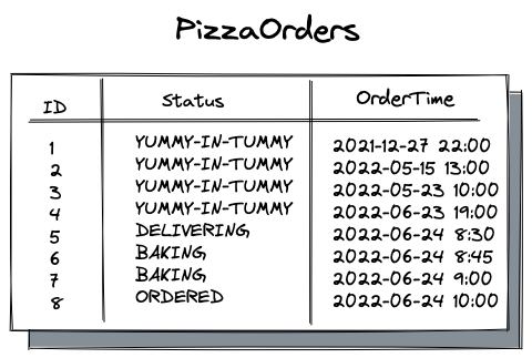
Each row in the table represents a customer order with a unique identifier (ID), the time the customer put the order in (OrderTime), and the current order’s Status. The status ranges from ORDERED to YUMMY-YUMMY-IN-MY-TUMMY. The latter status means that a pizza has already been delivered to the customer’s doors and, hopefully, consumed.
As a large pizza chain, the application needs to deal with thousands of orders daily. This means the size of the PizzaOrders table is getting out of control. Eventually, you take advantage of the table partitioning feature and split the table into several smaller independent tables called partitions.
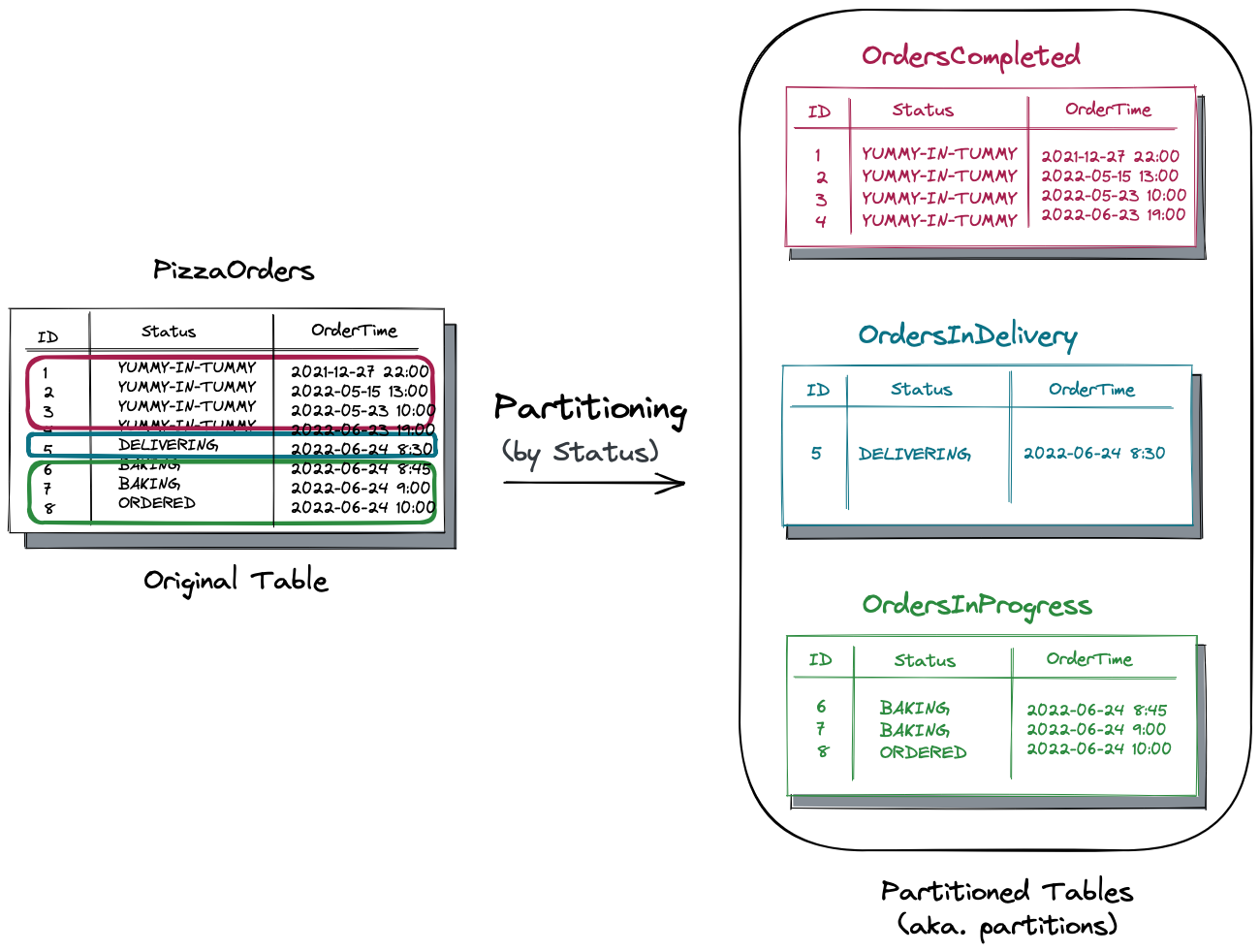
The original table gets split by the Status column into three partitioned tables:
- The
OrdersCompletedtable stores all the orders that were handed over to the customer. - The
OrdersInDeliverytracks the orders on the road to the customer’s location. - And the
OrdersInProgressis for the pizzas that are yet to be baked.
Nice! As a quick win, now you can manage the size and state of each partition independently and control the cost, for instance, by using a cheaper storage medium for historical data (OrdersCompleted). Also, you might see an immediate performance gain after the split for queries that request only pizzas with a specific status. For example, if the app requests all the orders that are in progress, then the request will go to the OrdersInProgress table, bypassing other partitions.
Alright, now you have a basic understanding of table partitioning. Next, let’s dive deeper and see how table partitioning can improve your apps’ performance. In this article, we start with the partition pruning feature.
Partition Pruning
In PostgreSQL, partition pruning is an optimization technique that allows the SQL engine to exclude unnecessary partitions from the execution. As a result, your query will run against a smaller data set, bypassing the excluded partitions. The smaller data set to query the better the performance.
Let’s see what happens when the planner and executor apply this optimization technique.
Creating Partitions
Earlier, we discussed how to use the status column to partition the PizzaOrders table into three tables: OrdersInProgress, OrdersInDelivery and OrdersCompleted. These are the DDL commands:
CREATE TYPE status_t AS ENUM('ordered', 'baking', 'delivering', 'yummy-in-my-tummy');

CREATE TABLE PizzaOrders
 (
   id   int,
   status   status_t,
   ordertime   timestamp,
   PRIMARY KEY (id, status)
 ) PARTITION BY LIST (status);

CREATE TABLE OrdersInProgress PARTITION OF PizzaOrders
  FOR VALUES IN('ordered','baking');

CREATE TABLE OrdersInDelivery PARTITION OF PizzaOrders
  FOR VALUES IN('delivering');

CREATE TABLE OrdersCompleted PARTITION OF PizzaOrders
  FOR VALUES IN('yummy-in-my-tummy');
The PARTITION BY LIST (status) clause requests to split the table using the List Partitioning method. With this method, the table is partitioned by explicitly listing which value(s) appear in each partition. PostgreSQL also supports Hash, Range, and Multilevel partitioning methods that you can review later.
After the split, you can use the command below to see the information about the table with its partitions:
\d+ PizzaOrders;

Partitioned table "public.pizzaorders"
  Column   |            Type             | Collation | Nullable | Default | Storage | Compression | Stats target | Description
-----------+-----------------------------+-----------+----------+---------+---------+-------------+--------------+-------------
 id        | integer                     |           | not null |         | plain   |             |              |
 status    | status_t                    |           | not null |         | plain   |             |              |
 ordertime | timestamp without time zone |           |          |         | plain   |             |              |
Partition key: LIST (status)
Indexes:
    "pizzaorders_pkey" PRIMARY KEY, btree (id, status)
Partitions: orderscompleted FOR VALUES IN ('yummy-in-my-tummy'),
            ordersindelivery FOR VALUES IN ('delivering'),
            ordersinprogress FOR VALUES IN ('ordered', 'baking')
Next, let’s insert sample data:
INSERT INTO PizzaOrders VALUES
(1, 'yummy-in-my-tummy', '2021-12-27 22:00:00'),
(2, 'yummy-in-my-tummy', '2022-05-15 13:00:00'),
(3, 'yummy-in-my-tummy', '2022-05-23 10:00:00'),
(4, 'yummy-in-my-tummy', '2022-06-23 19:00:00'),
(5, 'delivering', '2022-06-24 8:30:00'),
(6, 'baking', '2022-06-24 8:45:00'),
(7, 'baking', '2022-06-24 9:00:00'),
(8, 'ordered', '2022-06-24 10:00:00');
And run the query below to see in which partition each record is stored:
SELECT tableoid::regclass,* from PizzaOrders
  ORDER BY id;

     tableoid     | id |      status       |      ordertime
------------------+----+-------------------+---------------------
 orderscompleted  |  1 | yummy-in-my-tummy | 2021-12-27 22:00:00
 orderscompleted  |  2 | yummy-in-my-tummy | 2022-05-15 13:00:00
 orderscompleted  |  3 | yummy-in-my-tummy | 2022-05-23 10:00:00
 orderscompleted  |  4 | yummy-in-my-tummy | 2022-06-23 19:00:00
 ordersindelivery |  5 | delivering        | 2022-06-24 08:30:00
 ordersinprogress |  6 | baking            | 2022-06-24 08:45:00
 ordersinprogress |  7 | baking            | 2022-06-24 09:00:00
 ordersinprogress |  8 | ordered           | 2022-06-24 10:00:00
The tableoid column shows the name of a table that stores a respective record. As you can see, all the records were properly arranged across the partitioned tables based on the value of their Status column.
Partition Pruning in Action
Lastly, let’s assume you want to get all the orders that were handed over to customers and, hopefully, consumed by them:
EXPLAIN ANALYZE SELECT * FROM PizzaOrders
  WHERE status = 'yummy-in-my-tummy';

                                                           QUERY PLAN
--------------------------------------------------------------------------------------------------------------------------------
 Bitmap Heap Scan on orderscompleted pizzaorders  (cost=22.03..32.57 rows=9 width=16) (actual time=0.019..0.020 rows=4 loops=1)
   Recheck Cond: (status = 'yummy-in-my-tummy'::status_t)
   Heap Blocks: exact=1
   ->  Bitmap Index Scan on orderscompleted_pkey  (cost=0.00..22.03 rows=9 width=0) (actual time=0.012..0.013 rows=4 loops=1)
         Index Cond: (status = 'yummy-in-my-tummy'::status_t)
 Planning Time: 0.321 ms
 Execution Time: 0.052 ms
The execution plan shows that the query was executed over a single partition (OrdersCompleted) bypassing the others. This is the partition pruning feature in action! And it’s enabled by default in PostgreSQL.
Partition Pruning and Functions
Partition pruning works only if a query filters data by applying constant value or externally supplied parameters. If you try to use a non-immutable function within the WHERE clause section, the planner will skip this optimization and scan the entire table instead. Don’t be surprised if you see the following execution plan:
EXPLAIN ANALYZE SELECT * FROM PizzaOrders
  WHERE status::text = lower('yummy-in-my-tummy');

                                                           QUERY PLAN
--------------------------------------------------------------------------------------------------------------------------------
 Append  (cost=0.00..127.26 rows=27 width=16) (actual time=0.074..0.076 rows=4 loops=1)
   ->  Seq Scan on ordersinprogress pizzaorders_1  (cost=0.00..42.38 rows=9 width=16) (actual time=0.040..0.040 rows=0 loops=1)
         Filter: ((status)::text = 'yummy-in-my-tummy'::text)
         Rows Removed by Filter: 3
   ->  Seq Scan on ordersindelivery pizzaorders_2  (cost=0.00..42.38 rows=9 width=16) (actual time=0.019..0.019 rows=0 loops=1)
         Filter: ((status)::text = 'yummy-in-my-tummy'::text)
         Rows Removed by Filter: 1
   ->  Seq Scan on orderscompleted pizzaorders_3  (cost=0.00..42.38 rows=9 width=16) (actual time=0.014..0.015 rows=4 loops=1)
         Filter: ((status)::text = 'yummy-in-my-tummy'::text)
 Planning Time: 11.435 ms
 Execution Time: 0.222 ms
The planner doesn’t like guessing the time it might take to execute the function. Therefore, it queries all the partitions, which might be significantly faster.
To Be Continued…
Alright, that’s enough to understand the basics of table partitioning and how your apps can execute faster if the database applies the partition pruning optimization technique. What’s good about pruning is that you, as a developer, just define your tables and respective partitions, and then the database engine will take care of the optimization.
In the following articles, you’ll learn how partition management can simplify and improve the architecture of event-driven and streaming applications. You’ll also discover how you can use the geo-partitioning technique to pin user data to specific geographies. The latter method comes in handy when an app must comply with data regulatory requirements or serve user requests with low latency, regardless of the user’s location.


